EDGAR Filer Analysis

   

On this page:

• Data Sourcing and Preparation
  • Data Collection
  • Understanding Multiple Entities
  • Dataset Availability
  • Data Enrichment
• Getting Started
  • Augmenting with Sector & Industry Data
  • Augmenting with SIC Codes and SEC Offices
• Visualizing EDGAR Filers' Trends
• Sector and Industry Analysis of EDGAR Filers
  • Industry-Level Analysis
• EDGAR Entities by SIC and SEC Office

Welcome to the EDGAR Filer Analysis tutorial! Through this tutorial, we aim to offer a comprehensive overview of the trends and factors that have influenced the growth and fluctuations of entities on the SEC EDGAR platform from 1994 to 2022.

By employing various visualization techniques, we'll shed light on the number of EDGAR filers over this time span. Additionally, we'll enrich our dataset by incorporating sector and industry information, SIC codes, and the respective SEC office designations for each filer.

You'll get hands-on experience crafting stacked bar charts, line graphs, heatmaps, box plots, and more to unearth meaningful correlations and insights. Here's a sneak peek of the visualizations you're about to explore:

Below, we highlight some of the key observations and insights derived from the EDGAR filer statistics:

• Peak Filers: The year 2021 recorded the highest number of EDGAR filers ever.
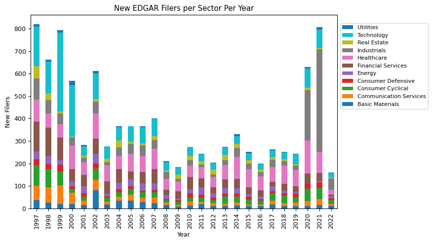
• Sectoral Growth: In 2021, there was a significant influx of new EDGAR filers, second only to 2003. Notably, the industrials and healthcare sectors observed the most pronounced growth.
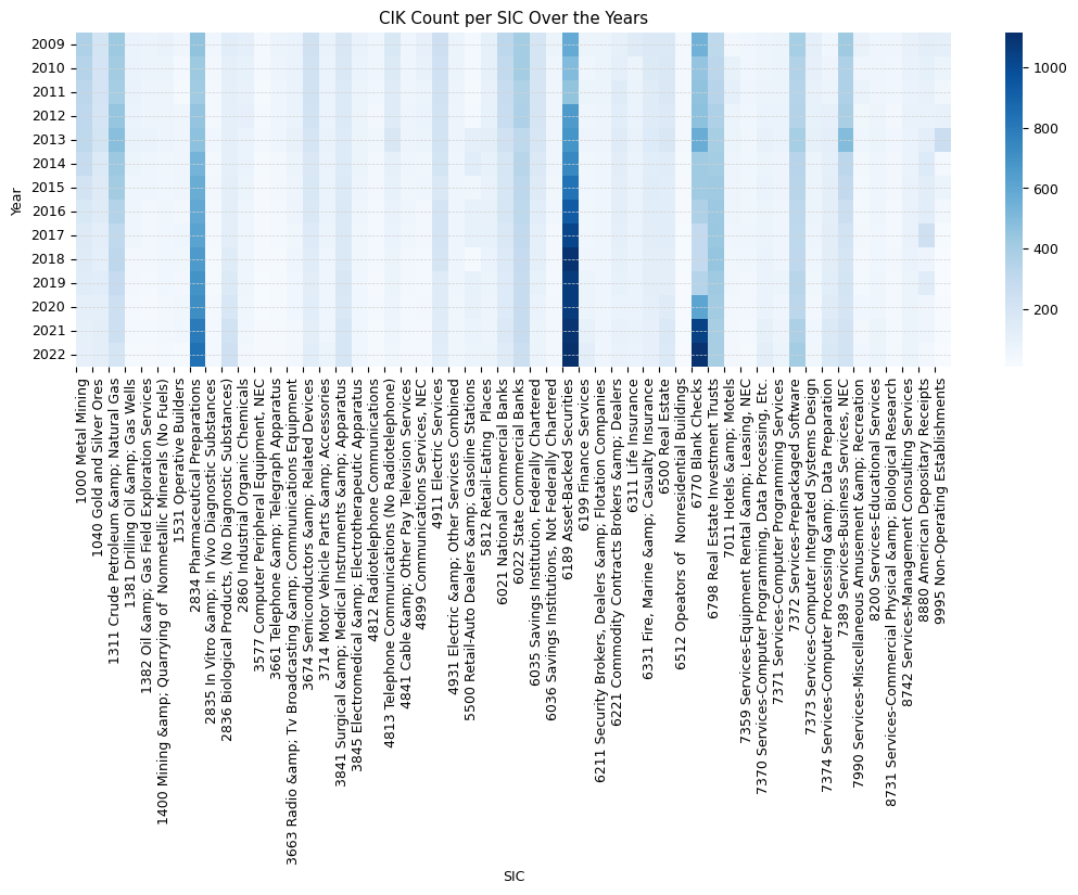
• SPAC Surge: A noticeable surge in Blank cheque companies (SPACs or shell companies) was evident between 2020 and 2022.
• Tech Sector Warning: There were anomalous increases in new tech sector filers between 1997 and 1999, hinting at the impending dot-com bubble of 2000.
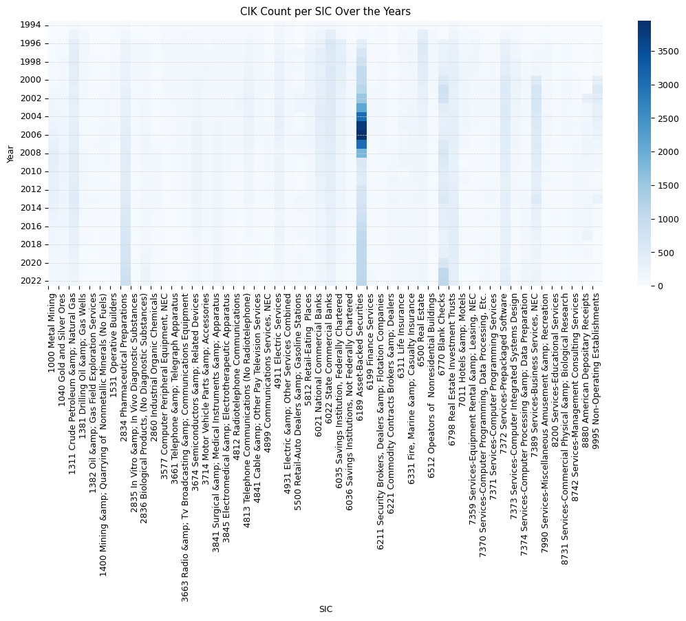
• Financial Crisis Precursor: Between 2003 and 2006, there was a spike in asset-backed securities – a potential early warning sign of the looming financial crisis.
• Assignment Trends: Over time, the number of new EDGAR filers linked to specific sectors or industries declined, while unassigned filers saw an uptick.
• SIC Code Omissions: Astonishingly, 90% of EDGAR filers are not assigned an SIC code, making them unlinked to any specific SEC office.
• Assignment Decline: Beginning in 2000, there was a consistent decline in the number of EDGAR filers associated with a sector, SIC code, or SEC office. This trend was counterbalanced by an increase in filers without any such affiliations.

Throughout this section, note that we use the terms filer and entity interchangeably.

The annual count of EDGAR filers was determined using the Query API. We extracted metadata for all EDGAR filings between 1994 and 2022, which included details like form type (e.g., 10-K) and filing entities (such as CIK, SIC, IRS number, and filer name). By referencing these entities in respective filings for each year, we compiled a comprehensive list. However, a deep dive into the aggregation process will not be covered here. Be prepared: executing the code responsible for this data collection and aggregation can span several days.

A single filing can encompass multiple entities. Take the insider trading form, Form 4, as an example. It always includes at least two entities: the issuer (the company issuing the securities) and the reporter (the individual or entity acquiring or disposing of the securities). Thus, one SEC Form 4 filing, with a unique accession number, results in two separate records in the EDGAR index—one for each entity. Here's an illustrative example showcasing Meta (formerly Facebook) and Mark Zuckerberg as the two entities:

Form 4 Example

On the other hand, S-4 filings can encompass even more entities. The following example houses nine distinct entities:

S-4 Filing Example

Key takeaways:

• A single filing can contain multiple entities.
• Every entity will possess a CIK and name, but not all will have an SIC code.

For the sake of convenience, we've prepared the entities dataset in advance. You can freely download the data from the following links:

• Entities from 1994 to 2011
• Entities from 2012 to 2022

The dataset structure is as follows:

{
  "2022": [
    {
      "cik": "789019",
      "companyName": "MICROSOFT CORP (Issuer)",
      "irsNo": "911144442",
      "fiscalYearEnd": "0630",
      "stateOfIncorporation": "WA",
      "sic": "7372 Services-Prepackaged Software",
      "year": "2022"
    },
    {
      "cik": "902012",
      "companyName": "GATES WILLIAM H III (Reporting)",
      "year": "2022"
    }
    // ... additional filers
  ]
  // ... other years
}

In the forthcoming steps, we will enhance our dataset by adding sector and industry data for each entity. This is achieved through the Mapping API, which links each entity's CIK to its corresponding sector and industry. If a mapping isn't available, the value will be represented as "NaN". Furthermore, we will associate the Standard Industrial Classification (SIC) codes of each entity to the appropriate SEC office, as detailed by the SEC's guidelines found here.

As we venture further into our EDGAR Filer Analysis, our next step is crucial: obtaining and processing our primary dataset. In this section, we will walk you through the process of:

1. Downloading the Entities Data: We'll programmatically fetch the entities.json files which house our essential data spanning from 1994 to 2022.
2. Conversion to a DataFrame: The raw JSON data will be transformed into a structured pandas DataFrame. This format is more conducive to the analytical operations we'll be performing.
3. Enriching the Data: We'll augment our dataset by appending sector, industry, and SEC office designations to each entity. This added information will give us a richer context as we delve deeper into our analysis.

By the end of this section, you'll have a robust, enriched dataset at your fingertips, ready for detailed exploration and visualization. Let's dive in!

!pip install -q sec-api

import pandas as pd
import numpy as np
import matplotlib.pyplot as plt
import matplotlib.ticker as mtick
import seaborn as sns
import json
import requests

plt.rcParams.update({'font.size': 9})

# load entities_1994_2011.json into entities_1994_2011 variable
url_a = "https://statistics.sec-api.io/tutorials/edgar-filer-analysis/entities_1994_2011.json"
response_a = requests.get(url_a)
entities_1994_2011 = response_a.json()

url_b = "https://statistics.sec-api.io/tutorials/edgar-filer-analysis/entities_2012_2022.json"
response_b = requests.get(url_b)
entities_2012_2022 = response_b.json()

# merge entities_1994_2011 and entities_2012_2022 into entities variable
entities_json = {**entities_1994_2011, **entities_2012_2022}

Next, we'll transform the list of entities from the JSON format into a pandas DataFrame. This DataFrame will feature the following columns: year, cik, irsNo, companyName, fiscalYearEnd, stateOfIncorporation, and sic.

def convert_json_to_dataframe(entities_json: dict) -> pd.DataFrame:
    entities_json_list = []

    for year in entities_json.keys():
        for entity in entities_json[year]:
            entity['cik'] = entity['cik'].lstrip('0')
            entity['year'] = year
            entities_json_list.append(entity)

    entities = pd.DataFrame(entities_json_list)

    return entities


entities = convert_json_to_dataframe(entities_json)
entities.drop(labels=['act', 'fileNo', 'type', 'filmNo'], axis=1, inplace=True)
year = entities['year']
entities.drop(labels=['year'], axis=1, inplace=True)
entities.insert(0, 'year', year)
entities['year'] = entities['year'].astype(int)

print('All EDGAR entities from 1994 - 2022')
entities # 3056738 rows

All EDGAR entities from 1994 - 2022

	year	fiscalYearEnd	stateOfIncorporation	cik	companyName	sic	irsNo
0	1994	1231	LA	96035	SYSTEM FUELS INC (Filer)	0000	NaN
1	1994	1130	NaN	89954	TRUST FOR SHORT TERM U S GOVERNMENT SECURITIES...	NaN	251289316
2	1994	0331	MA	901823	PUTNAM MANAGED HIGH YIELD TRUST (Filer)	0000	046733967
3	1994	1231	NY	872243	EMPIRE STATE MUNICIPAL EXEMPT TRUST GUARANTEED...	0000	NaN
4	1994	1231	NY	872246	EMPIRE STATE MUNICIPAL EXEMPT TRUST GUARANTEED...	0000	NaN
...	...	...	...	...	...	...	...
3056733	2022	1231	NY	1956590	GO UES Investors LLC (Filer)	NaN	920625088
3056734	2022	1231	T2	1955130	Broomfield International Ltd (Filed by)	NaN	000000000
3056735	2022	1231	DE	1895349	Bridger Healthcare SIV I, LP (Filer)	NaN	000000000
3056736	2022	NaN	NaN	1830807	Eden Douglas Todd (Filed by)	NaN	NaN
3056737	2022	NaN	DE	1895098	XN Opportunities IV LP (Filer)	NaN	000000000

3056738 rows × 7 columns

To further enrich our dataset, we'll incorporate sector and industry information for each entity using the Mapping API. Start by retrieving the mapping data for all CIKs available in the mapping database. Once obtained, we'll associate the CIKs from our entities DataFrame with their respective sectors and industries. This is achieved using pandas' df_A.merge(df_B) function, allowing us to seamlessly append the sector and industry columns to our DataFrame.

from sec_api import MappingApi

mappingApi = MappingApi(api_key='YOUR_API_KEY')

mappings_json = mappingApi.resolve('cik', '[0-9]')

mappings = pd.DataFrame(mappings_json).drop(columns=["id"])
mappings["cik"] = mappings["cik"].astype(str)
mappings[mappings["sector"] == ""] = np.nan
mappings[mappings["industry"] == ""] = np.nan

The mappings DataFrame comprises 16 columns. Among these, the cik, sector, and industry columns are most important for our analysis.

print(f"Number of mappings: {len(mappings)}")
mappings.head()

Number of mappings: 41847

	name	ticker	cik	cusip	exchange	isDelisted	category	sector	industry	sic	sicSector	sicIndustry	famaSector	famaIndustry	currency	location
0	AGILENT TECHNOLOGIES INC	A	1090872	00846U101	NYSE	False	Domestic Common Stock	Healthcare	Diagnostics & Research	3826	Manufacturing	Laboratory Analytical Instruments		Measuring and Control Equipment	USD	California; U.S.A
1	ALCOA CORP	AA	1675149	013872106	NYSE	False	Domestic Common Stock	Basic Materials	Aluminum	3334	Manufacturing	Primary Production Of Aluminum		Steel Works Etc	USD	Pennsylvania; U.S.A
2	ADMIRALTY BANCORP INC	AAAB	1066808	007231103	NASDAQ	True	Domestic Common Stock	Financial Services	Banks - Regional	6022	Finance Insurance And Real Estate	State Commercial Banks		Banking	USD	Florida; U.S.A
3	ALTANA AKTIENGESELLSCHAFT	AAAGY	1182802	02143N103	NYSE	True	ADR Common Stock	Healthcare	Biotechnology	2834	Manufacturing	Pharmaceutical Preparations		Pharmaceutical Products	EUR	Jordan
4	ADVANCED ACCELERATOR APPLICATIONS SA	AAAP	1611787	00790T100	NASDAQ	True	ADR Common Stock	Healthcare	Biotechnology	2834	Manufacturing	Pharmaceutical Preparations		Pharmaceutical Products	EUR	France

tmp_mappings = mappings.dropna(subset=['sector', 'industry'])
print(f"{len(entities)} filers before merging")
entities = entities.merge(tmp_mappings[['cik', 'sector', 'industry']].drop_duplicates(subset=['cik']), how='left', on='cik')
entities.drop_duplicates(inplace=True)
entities.reset_index(drop=True, inplace=True)
print(f"{len(entities)} filers after merging")

3056738 filers before merging
3056738 filers after merging

Upon merging the sector and industry data into our entities DataFrame, the final list of entities looks like this:

entities[entities['year']==2022].head()

	year	fiscalYearEnd	stateOfIncorporation	cik	companyName	sic	irsNo	sector	industry
2898221	2022	1231	DE	19617	JPMORGAN CHASE & CO (Filer)	6021 National Commercial Banks	132624428	Financial Services	Banks - Diversified
2898222	2022	1231	DE	1665650	JPMorgan Chase Financial Co. LLC (Filer)	6021 National Commercial Banks	475462128	NaN	NaN
2898223	2022	1231	X0	312070	BARCLAYS BANK PLC (Filer)	6029 Commercial Banks, NEC	000000000	NaN	NaN
2898224	2022	NaN	NaN	1504477	Blend L Michael (Reporting)	NaN	NaN	NaN	NaN
2898225	2022	1231	DE	1805833	System1, Inc. (Issuer)	7370 Services-Computer Programming, Data Proce...	981531250	Industrials	Specialty Business Services

Our next enhancement involves associating SIC codes with their respective SEC Offices. Fortunately, the SEC website provides a detailed mapping between SIC codes and SEC offices, which can be found here: SEC SIC Code List.

For ease of access, we've already extracted and converted this mapping, inclusive of SIC codes, SEC office designations, and industry titles, into a JSON file. You can fetch it directly from: SIC-to-Office Mapping JSON.

In this section, we'll:

1. Download the provided JSON file.
2. Separate the SIC column in our entities DataFrame into two distinct columns: sic_code (housing the 3-4 digit code) and sic_industry (containing the industry title).
3. Integrate the SIC-to-Office mapping with our entities DataFrame.

Post these steps, our enriched entities DataFrame will feature an additional office column, indicating the designated SEC office for each entry.

sic_code_url = "https://statistics.sec-api.io/tutorials/edgar-filer-analysis/sic-codes-list.json"
sic_code_response = requests.get(sic_code_url)
sic_codes_json = sic_code_response.json()

sic_codes = pd.DataFrame(sic_codes_json)
sic_codes['sic_code'] = sic_codes['sic_code'].astype(str)

sic_codes

	sic_code	office	industry_title
0	100	Industrial Applications and Services	AGRICULTURAL PRODUCTION-CROPS
1	200	Industrial Applications and Services	AGRICULTURAL PROD-LIVESTOCK & ANIMAL SPECIALTIES
2	700	Industrial Applications and Services	AGRICULTURAL SERVICES
3	800	Industrial Applications and Services	FORESTRY
4	900	Industrial Applications and Services	FISHING, HUNTING AND TRAPPING
...	...	...	...
439	8880	Office of International Corp Fin	AMERICAN DEPOSITARY RECEIPTS
440	8888	Office of International Corp Fin	FOREIGN GOVERNMENTS
441	8900	Office of Trade & Services	SERVICES-SERVICES, NEC
442	9721	Office of International Corp Fin	INTERNATIONAL AFFAIRS
443	9995	Office of Real Estate & Construction	NON-OPERATING ESTABLISHMENTS

444 rows × 3 columns

# split "sic" column in sic_stats into "sic_code" and "sic_industry" columns by splitting at first space
entities[['sic_code', 'sic_industry']] = entities['sic'].str.split(n=1, expand=True)
entities['sic_code'] = entities['sic_code'].str.lstrip('0')
entities['sic_code'].replace('', np.nan, inplace=True)
entities['sic_industry'].replace({None: np.nan}, inplace=True)

print(f"{len(entities)} filers before merging")
entities = entities.merge(sic_codes[['sic_code', 'office']], how='left', on='sic_code')
entities.reset_index(drop=True, inplace=True)
print(f"{len(entities)} filers after merging")

3056738 filers before merging
3056738 filers after merging

We're set! Our entities DataFrame now encompasses sector and industry details for each EDGAR entity, complemented by the designated SEC Office, SIC code, and SIC industry title. With this enriched dataset in hand, we're ready to delve into visualization and analysis.

entities[entities['year']==2022].head()

	year	fiscalYearEnd	stateOfIncorporation	cik	companyName	sic	irsNo	sector	industry	sic_code	sic_industry	office
2898221	2022	1231	DE	19617	JPMORGAN CHASE & CO (Filer)	6021 National Commercial Banks	132624428	Financial Services	Banks - Diversified	6021	National Commercial Banks	Office of Finance
2898222	2022	1231	DE	1665650	JPMorgan Chase Financial Co. LLC (Filer)	6021 National Commercial Banks	475462128	NaN	NaN	6021	National Commercial Banks	Office of Finance
2898223	2022	1231	X0	312070	BARCLAYS BANK PLC (Filer)	6029 Commercial Banks, NEC	000000000	NaN	NaN	6029	Commercial Banks, NEC	Office of Finance
2898224	2022	NaN	NaN	1504477	Blend L Michael (Reporting)	NaN	NaN	NaN	NaN	NaN	NaN	NaN
2898225	2022	1231	DE	1805833	System1, Inc. (Issuer)	7370 Services-Computer Programming, Data Proce...	981531250	Industrials	Specialty Business Services	7370	Services-Computer Programming, Data Processing...	Office of Technology

It's time to bring our data to life through visualization. In this section, we'll illustrate the trajectory of EDGAR filers over the years.

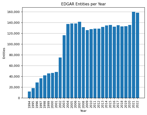
1. Annual EDGAR Filers: A bar chart will showcase the number of entities that filed an EDGAR filing from 1994 to 2022.
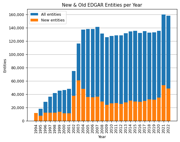
2. New vs. Total Filers: We'll compute the yearly count of new EDGAR filers and contrast this against the cumulative total using compelling visuals.
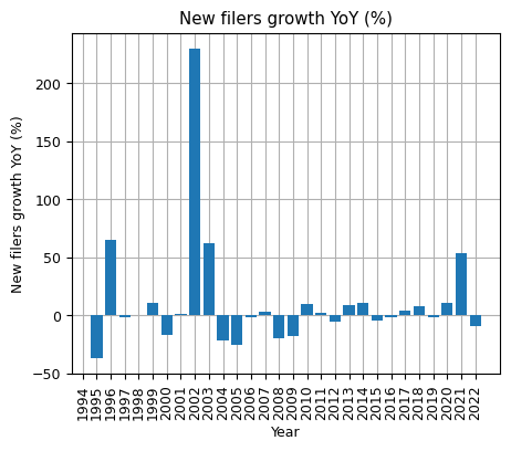
3. Growth Analysis: To further understand the dynamics, we'll calculate and visualize the year-on-year percentage growth in new filers.

These visualizations will not only offer a bird's-eye view of the trends but also equip us with insights into the nuances of filer growth and the factors influencing them.

years = entities['year'].unique().tolist()
num_entities = entities.groupby('year').size().tolist()

plt.bar(years, num_entities)
plt.xlabel('Year'), plt.ylabel('Entities'), plt.title('EDGAR Entities per Year')
ax = plt.gca()
ax.yaxis.set_major_formatter(mtick.FuncFormatter(lambda x, p: format(int(x), ',')))
plt.xticks(years, rotation=90), plt.grid(axis='y'), plt.gca().set_axisbelow(True)
plt.show()

Let us now find entities that are seen for the first time in each year, allowing us to track when each entity first appeared in the dataset.

For this, we define the function get_new_filers_per_year that processes the entities dataframe to identify new entities (or 'filers') for each year, i.e., entities that are seen for the first time in that year.

def get_new_filers_per_year(entities):
    new_filers = None
    processed_ciks = set()
    years = entities['year'].unique().tolist()

    for year in years:
        ciks = entities[entities['year'] == year]['cik'].tolist()
        if year == 1994:
            new_filers = pd.DataFrame(entities[entities['year'] == year])
            processed_ciks.update(ciks)
            continue

        year_entities = entities[entities['year'] == year]
        new_filers_for_year = year_entities[~year_entities['cik'].isin(processed_ciks)]
        new_filers = pd.concat([new_filers, new_filers_for_year], ignore_index=True)

        processed_ciks.update(ciks)

    return new_filers

new_filers = get_new_filers_per_year(entities)

print('New EDGAR entities in 2020:', len(new_filers[new_filers['year'] == 2020])) # 35055

New EDGAR entities in 2020: 35055

The next code snippet is designed to visualize the distribution of entities over the years, specifically highlighting the difference between all entities and the new entities added each year.

years = entities['year'].unique().tolist()
num_entities = entities.groupby('year').size().tolist()
num_new_filers = new_filers.groupby('year').size().tolist()

plt.bar(years, num_entities, label='All entities')
plt.bar(years, num_new_filers, label='New entities')
plt.xlabel('Year'), plt.ylabel('Entities'), plt.title('New & Old EDGAR Entities per Year')
plt.legend()
ax = plt.gca()
ax.yaxis.set_major_formatter(mtick.FuncFormatter(lambda x, p: format(int(x), ',')))
plt.xticks(years, rotation=90), plt.grid(axis='y'), plt.gca().set_axisbelow(True)
plt.show()

years = entities['year'].unique().tolist()

filers_df = pd.DataFrame({'total filers': num_entities, 'new filers': num_new_filers}, index=sorted(years))
filers_df['new filers %'] = filers_df['new filers'] / filers_df['total filers'] * 100
filers_df['new filers %'] = filers_df['new filers %'].map('{:,.1f}'.format)
filers_df['filers growth YoY'] = filers_df['total filers'].pct_change() * 100
filers_df['filers growth YoY'] = filers_df['filers growth YoY'].map('{:,.1f}'.format)
filers_df['new filers growth YoY'] = filers_df['new filers'].pct_change() * 100
filers_df['new filers growth YoY'] = filers_df['new filers growth YoY'].map('{:,.1f}'.format)
filers_df = filers_df.sort_index(ascending=False)

filers_df.head()

	total filers	new filers	new filers %	filers growth YoY	new filers growth YoY
2022	158517	48682	30.7	-1.0	-9.4
2021	160186	53713	33.5	18.3	53.2
2020	135393	35055	25.9	1.4	10.3
2019	133494	31783	23.8	0.5	-1.2
2018	132826	32173	24.2	-1.7	7.9

filers_df['new filers growth YoY'] = filers_df['new filers growth YoY'].astype(float)
plt.figure(figsize=(5, 4)), plt.bar(filers_df.index, filers_df['new filers growth YoY'])
plt.title('New filers growth YoY (%)'), plt.xlabel('Year'), plt.ylabel('New filers growth YoY (%)')
plt.grid(axis='y'), plt.grid(axis='x')
plt.gca().set_axisbelow(True), plt.xticks(filers_df.index, rotation=90)
plt.show()

Let's summarize the insights from the EDGAR filer's data so far collected:

1. The year 2021 marked an all-time high in the number of EDGAR entities, reaching a pinnacle of 160,186 filers. The year recorded a 53% surge in new filers relative to 2020.
2. 2021 recorded the second-highest count of newcomers to the EDGAR platform.
3. While 2022 experienced a slight dip in new filers compared to its preceding year, it still ranks third in the all-time highest new filer counts.
4. Despite the challenges of the COVID-19 pandemic in 2020, both new and total EDGAR filers saw an upward trend compared to 2019.
5. The record for the most significant number of new filers goes to 2003, standing second only to 2021, while 2002 witnessed a staggering 230% growth in new filers when contrasted with 2001. It's worth noting that the subsequent year, 2004, witnessed the enforcement of the Sarbanes-Oxley Act, which augmented reporting norms for public entities. This legislative change possibly fueled the surge in new filers in 2003.
6. The global financial crisis had a visible impact on EDGAR's metrics. For the first time since EDGAR's inception in 1994, the total number of entities declined during 2008 and 2009.
7. A consistent year-on-year decrease in new filers was observed from 2003 to 2009.
8. Post-2009, from 2010 onwards, there has been a gradual year-on-year increase in both new and overall entities on EDGAR.

In this section, we'll focus on a detailed analysis of EDGAR filers segmented by sectors and industries from 1994 to 2022. Our approach will involve:

1. Data Segmentation: Utilizing pivot tables, we'll categorize the number of EDGAR filers per sector and industry over the specified timeframe.
2. Visualization: Stacked bar charts and line charts will be employed to represent the distribution and trends of filers across different sectors and industries.
3. Anomaly Detection: We'll also examine the data for any anomalies which might indicate underlying market trends or significant events.

sector_stats = entities.groupby(['year', 'sector'], dropna=False).cik.count().reset_index(name='cik_count')
sector_stats[sector_stats['year'] == 2022].sort_values(by='cik_count', ascending=False).head(20)

	year	sector	cik_count
347	2022	NaN	151476
342	2022	Healthcare	1461
343	2022	Industrials	1360
345	2022	Technology	934
341	2022	Financial Services	921
338	2022	Consumer Cyclical	631
336	2022	Basic Materials	374
344	2022	Real Estate	315
340	2022	Energy	308
337	2022	Communication Services	303
339	2022	Consumer Defensive	296
346	2022	Utilities	138

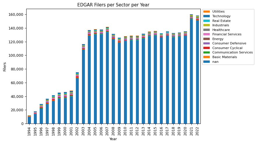
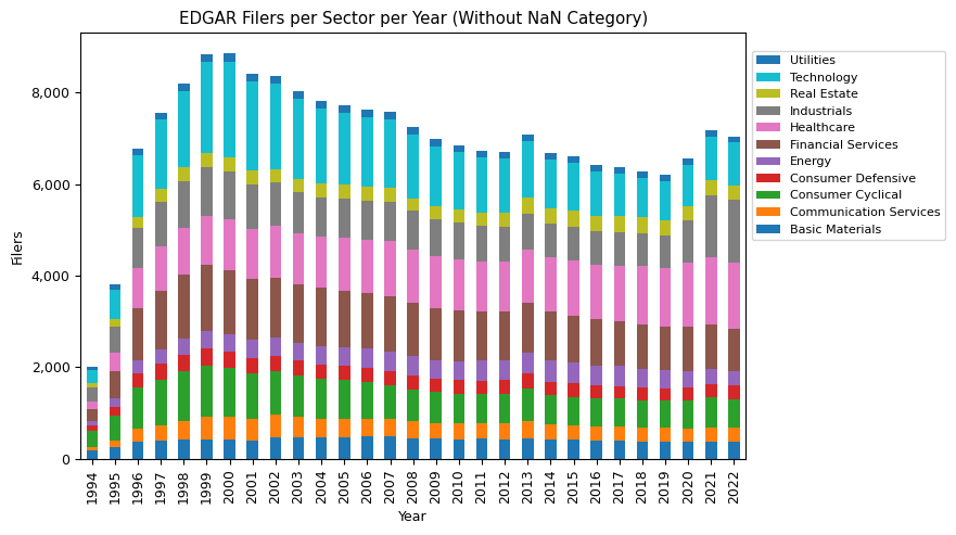
We've segmented the data into 12 unique sectors, one of which is the 'NaN' category. This category encompasses entities that haven't been designated a specific sector, such as trusts or insiders often documented in Form 4.

From the 2022 snapshot generated, we can observe the distribution of EDGAR filers across these 12 sectors. The 'NaN' category stands out with a substantial count of 151,477 entities. However, looking beyond this, the 'Healthcare' sector is prominently represented with 1,461 entities, closely trailed by the 'Industrials' sector with 1,360 entities. Such figures indicate a high level of activity and growth in these sectors. Additionally, the 'Technology' and 'Financial Services' sectors remain influential with 934 and 920 entities, respectively. On the other end of the spectrum, the strictly regulated 'Utilities' sector has the least presence, with only 138 entities for 2022.

To examine the distribution of filers across sectors over the years, we construct a pivot table. This table designates years as the index column and sectors as column labels. Each cell within this matrix indicates the quantity of EDGAR filers corresponding to a specific sector for a particular year.

sector_stats_pivot = sector_stats.pivot(index='year', columns='sector', values='cik_count')
sector_stats_pivot[-10:]

sector	NaN	Basic Materials	Communication Services	Consumer Cyclical	Consumer Defensive	Energy	Financial Services	Healthcare	Industrials	Real Estate	Technology	Utilities
year
2013	124658	452	370	725	311	453	1087	1158	800	337	1250	140
2014	128024	426	324	639	296	455	1078	1178	744	337	1062	146
2015	129015	415	310	622	296	451	1035	1203	742	343	1040	148
2016	126135	407	300	612	281	430	1019	1185	731	340	966	150
2017	128784	402	301	608	280	433	980	1213	738	340	920	151
2018	126555	387	295	599	268	415	978	1272	718	335	861	143
2019	127300	378	295	604	270	387	941	1292	719	325	848	135
2020	128845	364	302	621	276	361	955	1403	918	320	891	137
2021	153015	375	319	644	297	339	954	1485	1344	318	958	138
2022	151476	374	303	631	296	308	921	1461	1360	315	934	138

Let's start by visualizing the data to get a clearer sense of the trends. Once we have the visual representation, we can identify and list the key insights.

sector_stats_pivot.plot(kind='bar', stacked=True, figsize=(7, 5))
plt.title("EDGAR Filers per Sector per Year")
plt.ylabel("Filers"), plt.xlabel("Year"), plt.tight_layout()
ax = plt.gca()
ax.yaxis.set_major_formatter(mtick.FuncFormatter(lambda x, p: format(int(x), ',')))
handles, labels = ax.get_legend_handles_labels()
ax.legend(reversed(handles), reversed(labels), loc='lower left', bbox_to_anchor=(1, 0.5), fontsize=8)
plt.show()

sector_stats_pivot.drop(columns=[np.nan]).plot(kind='bar', stacked=True, figsize=(7, 5))
plt.title("EDGAR Filers per Sector per Year (Without NaN Category)")
plt.ylabel("Filers"), plt.xlabel("Year"), plt.tight_layout()
ax = plt.gca()
ax.yaxis.set_major_formatter(mtick.FuncFormatter(lambda x, p: format(int(x), ',')))
handles, labels = ax.get_legend_handles_labels()
ax.legend(reversed(handles), reversed(labels), loc='lower left', bbox_to_anchor=(1, 0.5), fontsize=8)
plt.show()

sector_stats_pivot.drop(columns=[np.nan]).plot(kind='line', figsize=(7, 5))
plt.title("EDGAR Filers per Sector per Year")
plt.ylabel("Filers"), plt.xlabel("Year"), plt.tight_layout(), plt.grid(True), plt.gca().set_axisbelow(True)
plt.xticks(sector_stats_pivot.index, rotation=90)
ax = plt.gca()
ax.yaxis.set_major_formatter(mtick.FuncFormatter(lambda x, p: format(int(x), ',')))
handles, labels = ax.get_legend_handles_labels()
ax.legend(reversed(handles), reversed(labels), loc='lower left', bbox_to_anchor=(1, 0.5), fontsize=8)
plt.show()

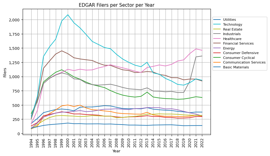
From the visual representation of the EDGAR filers per sector over time, we can derive the following key insights:

1. Technology Boom and Subsequent Stabilization: The Technology sector experienced a significant rise in the number of filers from 1996 to 2000, likely corresponding to the dot-com boom. However, after 2000, there was a decline, and then the number of filers stabilized and even increased slightly in the most recent years.

2. Financial Services Peak and Decline: The Financial Services sector saw a steady increase in the number of filers up to around 1999, after which there was a gradual decline, with minor fluctuations in the subsequent years.

3. Healthcare's Consistent Rise: The Healthcare sector has experienced a consistent increase in the number of filers over the years, with notable growth in the most recent years.

4. Consumer Cyclical Variability: The Consumer Cyclical sector experienced a steady rise until around 1999, followed by a decline. The sector has seen fluctuations but remains one of the larger sectors in terms of filers.

5. Stability in Utilities: The Utilities sector has remained relatively stable over the years in terms of the number of filers.

6. Industrials' Recent Surge: The Industrials sector has seen a significant rise in the number of filers in the last couple of years, indicating recent activity or interest in this sector.

7. General Sector Trends: Most sectors experienced growth in the number of filers during the mid to late 90s, followed by stabilization or slight decline in the 2000s. The past decade has seen either stabilization or growth for many sectors, with some exceptions.

8. Smallest Sectors: Communication Services and Real Estate have consistently been among the sectors with the lowest number of filers, though they too have experienced fluctuations over the years.

9. Impact of Global Events: Notable declines in many sectors can be observed around 2008, likely corresponding to the global financial crisis.

These insights provide a high-level view of the trends and shifts in the different sectors over the years based on the EDGAR filers' data. Further analysis could delve deeper into the reasons behind these trends, especially the recent surge in the Industrials sector.

sector_stats_new_filers = new_filers.groupby(['year', 'sector'], dropna=False).cik.count().reset_index(name='cik_count')
sector_stats_new_filers[sector_stats_new_filers['year'] == 2022].sort_values(by='cik_count', ascending=False).head(20)

	year	sector	cik_count
346	2022	NaN	48522
342	2022	Industrials	51
341	2022	Healthcare	21
344	2022	Technology	21
337	2022	Consumer Cyclical	18
335	2022	Basic Materials	11
336	2022	Communication Services	9
339	2022	Energy	9
340	2022	Financial Services	8
338	2022	Consumer Defensive	7
343	2022	Real Estate	3
345	2022	Utilities	2

sector_stats_new_filers_pivot = sector_stats_new_filers.pivot(index='year', columns='sector', values='cik_count')
sector_stats_new_filers_pivot.fillna(0, inplace=True)
sector_stats_new_filers_pivot = sector_stats_new_filers_pivot.astype(int)
sector_stats_new_filers_pivot[-5:]

sector	NaN	Basic Materials	Communication Services	Consumer Cyclical	Consumer Defensive	Energy	Financial Services	Healthcare	Industrials	Real Estate	Technology	Utilities
year
2018	31920	10	14	33	11	10	31	81	21	7	32	3
2019	31539	11	15	24	17	7	25	71	21	7	44	2
2020	34426	10	22	56	21	1	45	147	225	11	85	6
2021	52907	15	26	50	24	8	34	96	456	5	83	9
2022	48522	11	9	18	7	9	8	21	51	3	21	2

sector_stats_new_filers_pivot.loc[1997:, :].drop(columns=[np.nan]).plot(kind='bar', stacked=True, figsize=(7, 5))
plt.title("New EDGAR Filers per Sector Per Year"), plt.ylabel("New Filers"), plt.xlabel("Year"), plt.tight_layout()
ax = plt.gca()
ax.yaxis.set_major_formatter(mtick.FuncFormatter(lambda x, p: format(int(x), ',')))
handles, labels = ax.get_legend_handles_labels()
ax.legend(reversed(handles), reversed(labels), loc='lower left', bbox_to_anchor=(1, 0.5), fontsize=8)
plt.show()

Building on our sectorial analysis, we now narrow our focus to the industry level, offering a more granular perspective on the landscape of EDGAR filers over last three decades.

While bar charts will provide a clear representation of the data, we'll also introduce heatmaps to capture and visualize correlations between industries. Such visual tools offer a nuanced understanding of industry interplay and their respective prominence over time.

industry_stats = entities.groupby(['year', 'industry'], dropna=False).cik.count().reset_index(name='cik_count')
industry_stats[industry_stats['year'] == 2022].sort_values(by='cik_count', ascending=False).head(10)

	year	industry	cik_count
4360	2022	NaN	151476
4230	2022	Biotechnology	831
4334	2022	Shell Companies	644
4226	2022	Banks - Regional	417
4336	2022	Software - Application	317
4292	2022	Medical Devices	181
4337	2022	Software - Infrastructure	165
4220	2022	Asset Management	141
4252	2022	Drug Manufacturers - Specialty & Generic	115
4298	2022	Oil & Gas E&P	103

print('Number of industries:', len(industry_stats['industry'].unique()))

Number of industries: 154

industry_stats_pivot = industry_stats.pivot(index='year', columns='industry', values='cik_count')
industry_stats_pivot.fillna(0, inplace=True)
industry_stats_pivot = industry_stats_pivot.astype(int)
industry_stats_pivot[-5:]

industry	NaN	Advertising Agencies	Aerospace & Defense	Agricultural Inputs	Airlines	Airports & Air Services	Aluminum	Apparel Manufacturing	Apparel Retail	Asset Management	...	Travel Services	Trucking	Uranium	Utilities - Diversified	Utilities - Independent Power Producers	Utilities - Regulated Electric	Utilities - Regulated Gas	Utilities - Regulated Water	Utilities - Renewable	Waste Management
year
2018	126555	41	64	22	24	10	6	25	46	136	...	15	21	10	14	9	68	23	17	12	25
2019	127300	42	64	17	24	10	6	23	43	137	...	20	21	10	14	8	62	20	18	13	29
2020	128845	45	73	17	25	10	6	22	44	145	...	21	23	8	15	9	60	19	16	18	30
2021	153015	52	79	17	25	12	6	25	41	149	...	20	21	9	15	7	57	19	17	23	27
2022	151476	51	79	19	25	12	6	23	37	141	...	18	22	10	15	7	56	19	16	25	26

5 rows × 154 columns

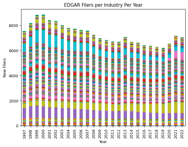
industry_stats_pivot.loc[1997:, :].drop(columns=[np.nan]).plot(kind='bar', stacked=True, figsize=(7, 5))
plt.title("EDGAR Filers per Industry Per Year")
plt.ylabel("New Filers"), plt.xlabel("Year"), plt.legend().set_visible(False)
plt.show()

industry_stats_new_filers = new_filers.groupby(['year', 'industry'], dropna=False).cik.count().reset_index(name='cik_count')
industry_stats_pivot_new_filers = industry_stats_new_filers.pivot(index='year', columns='industry', values='cik_count')
industry_stats_pivot_new_filers.fillna(0, inplace=True)
industry_stats_pivot_new_filers = industry_stats_pivot_new_filers.astype(int)
industry_stats_pivot_new_filers[-5:]

industry	NaN	Advertising Agencies	Aerospace & Defense	Agricultural Inputs	Airlines	Airports & Air Services	Aluminum	Apparel Manufacturing	Apparel Retail	Asset Management	...	Travel Services	Trucking	Uranium	Utilities - Diversified	Utilities - Independent Power Producers	Utilities - Regulated Electric	Utilities - Regulated Gas	Utilities - Regulated Water	Utilities - Renewable	Waste Management
year
2018	31920	1	0	2	1	1	0	1	0	3	...	0	0	1	0	0	0	2	0	1	1
2019	31539	2	3	2	0	1	0	0	1	5	...	0	1	0	0	0	0	1	0	1	2
2020	34426	3	9	1	0	2	0	0	1	10	...	2	1	0	1	0	0	0	0	5	0
2021	52907	7	9	0	0	2	0	2	1	8	...	0	0	0	0	0	0	1	1	7	2
2022	48522	1	2	2	0	1	0	0	0	1	...	0	1	1	0	0	0	0	0	2	2

5 rows × 154 columns

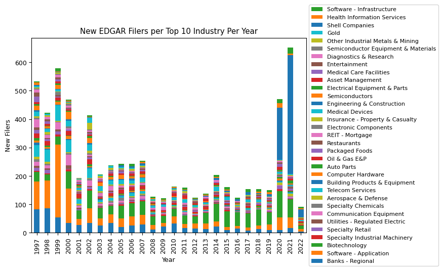
top_10_industries = {}
for year in range(1994, 2023):
    top_10_industries[year] = industry_stats_new_filers[industry_stats_new_filers['year'] == year].sort_values(by='cik_count', ascending=False).head(20)
    top_10_industries[year] = top_10_industries[year][top_10_industries[year]['cik_count'] > 15]

top_10_industries_df = pd.concat(top_10_industries, axis=0)
top_10_industries_df.reset_index(inplace=True)
top_10_industries_df.drop(columns=['level_0', 'level_1'], inplace=True)
top_10_industries_df['year'] = top_10_industries_df['year'].astype(int)
top_10_industries_df

	year	industry	cik_count
0	1994	NaN	9915
1	1994	Banks - Regional	137
2	1994	Software - Application	65
3	1994	Biotechnology	63
4	1994	Specialty Industrial Machinery	59
...	...	...	...
171	2021	Software - Application	38
172	2021	Software - Infrastructure	22
173	2021	Banks - Regional	16
174	2022	NaN	48522
175	2022	Shell Companies	29

176 rows × 3 columns

top_10_industries_df = top_10_industries_df['industry'].unique().tolist()

industry_stats_pivot_new_filers_top_10 = industry_stats_pivot_new_filers[top_10_industries_df]

industry_stats_pivot_new_filers_top_10.loc[1997:, :].drop(columns=[np.nan]).plot(kind='bar', stacked=True, figsize=(7, 5))
plt.title("New EDGAR Filers per Top 10 Industry Per Year"), plt.ylabel("New Filers"), plt.xlabel("Year")
ax = plt.gca()
handles, labels = ax.get_legend_handles_labels()
ax.legend(reversed(handles), reversed(labels), loc='center left', bbox_to_anchor=(1, 0.5), fontsize=8)
plt.show()

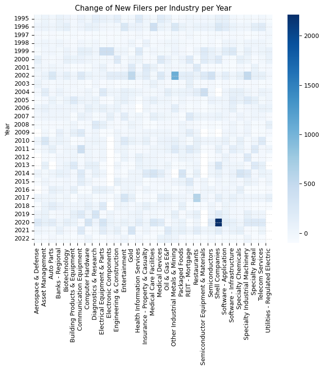
industry_stats_pivot_new_filers_top_10_pct_change = industry_stats_pivot_new_filers_top_10.pct_change() * 100
industry_stats_pivot_new_filers_top_10_pct_change = industry_stats_pivot_new_filers_top_10_pct_change.iloc[1:, :]
industry_stats_pivot_new_filers_top_10_pct_change = industry_stats_pivot_new_filers_top_10_pct_change.replace([np.inf, -np.inf], 0)
industry_stats_pivot_new_filers_top_10_pct_change = industry_stats_pivot_new_filers_top_10_pct_change.iloc[:, 1:]
industry_stats_pivot_new_filers_top_10_pct_change = industry_stats_pivot_new_filers_top_10_pct_change.reindex(sorted(industry_stats_pivot_new_filers_top_10_pct_change.columns), axis=1)
industry_stats_pivot_new_filers_top_10_pct_change[-5:]

industry	Aerospace & Defense	Asset Management	Auto Parts	Banks - Regional	Biotechnology	Building Products & Equipment	Communication Equipment	Computer Hardware	Diagnostics & Research	Electrical Equipment & Parts	...	Semiconductor Equipment & Materials	Semiconductors	Shell Companies	Software - Application	Software - Infrastructure	Specialty Chemicals	Specialty Industrial Machinery	Specialty Retail	Telecom Services	Utilities - Regulated Electric
year
2018	-100.000000	50.000000	150.000000	62.500000	12.000000	0.000000	0.000000	100.0	0.0	200.000000	...	-100.0	0.000000	-66.666667	30.000000	-18.181818	-50.0	-50.000000	-100.000000	-100.000000	-100.0
2019	0.000000	66.666667	-60.000000	-30.769231	-23.214286	100.000000	200.000000	0.0	300.0	-66.666667	...	NaN	0.000000	166.666667	46.153846	-22.222222	-50.0	100.000000	0.000000	0.000000	NaN
2020	200.000000	100.000000	150.000000	0.000000	116.279070	50.000000	-66.666667	300.0	25.0	300.000000	...	NaN	200.000000	2212.500000	136.842105	85.714286	0.0	200.000000	225.000000	200.000000	NaN
2021	0.000000	-20.000000	-40.000000	77.777778	-31.182796	-66.666667	200.000000	-87.5	-40.0	150.000000	...	0.0	33.333333	125.945946	-15.555556	69.230769	100.0	-66.666667	-76.923077	33.333333	NaN
2022	-77.777778	-87.500000	-33.333333	-75.000000	-79.687500	-100.000000	-66.666667	0.0	-100.0	-100.000000	...	-100.0	-50.000000	-93.062201	-76.315789	-77.272727	-100.0	0.000000	-100.000000	-100.000000	NaN

5 rows × 33 columns

sns.heatmap(industry_stats_pivot_new_filers_top_10_pct_change, cmap='Blues')
plt.gcf().set_size_inches(7, 7), plt.title("Change of New Filers per Industry per Year")
plt.ylabel("Year"), plt.xlabel(""), plt.tight_layout(), plt.grid(color='lightgrey', linestyle='dashed', linewidth=0.5)
ax = plt.gca()
ax.tick_params(axis='x', rotation=50), ax.set_xticklabels(ax.get_xticklabels(), ha='left')
plt.xticks(np.arange(len(industry_stats_pivot_new_filers_top_10_pct_change.columns)), industry_stats_pivot_new_filers_top_10_pct_change, rotation=90)
plt.yticks(np.arange(0.5, len(industry_stats_pivot_new_filers_top_10_pct_change.loc[1995:, :].index), 1), industry_stats_pivot_new_filers_top_10_pct_change.loc[1995:, :].index, rotation=0)
plt.show()

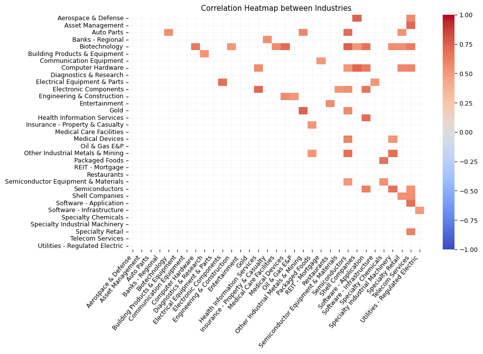
industry_stats_pivot_new_filers_top_10_corr = industry_stats_pivot_new_filers_top_10_pct_change.corr()
industry_stats_pivot_new_filers_top_10_corr = industry_stats_pivot_new_filers_top_10_corr[(industry_stats_pivot_new_filers_top_10_corr > 0.5) | (industry_stats_pivot_new_filers_top_10_corr < -0.5)]
# hide all values below the diagonal
mask = np.tril(np.ones_like(industry_stats_pivot_new_filers_top_10_corr, dtype=bool))
plt.figure(figsize=(12, 10))
sns.heatmap(industry_stats_pivot_new_filers_top_10_corr, annot=False, cmap='coolwarm', vmin=-1, vmax=1, mask=mask)
plt.title('Correlation Heatmap between Industries'), plt.tight_layout(), plt.gcf().set_size_inches(10, 7)
plt.ylabel(''), plt.xlabel('')
plt.gca().xaxis.grid(color='lightgrey', linestyle='dashed', linewidth=0.5, which='major', alpha=0.5)
plt.gca().yaxis.grid(color='lightgrey', linestyle='dashed', linewidth=0.5, which='major', alpha=0.5)
plt.gca().set_axisbelow(True)
ax = plt.gca()
ax.tick_params(axis='x', rotation=50), ax.set_xticklabels(ax.get_xticklabels(), ha='right')
plt.show()

most_correlated_industries = industry_stats_pivot_new_filers_top_10_corr.sum().sort_values(ascending=False).head(10)
print('Top 10 industries correlated the most with the other industries')
print('-'*70)
most_correlated_industries

Top 10 industries correlated the most with the other industries
----------------------------------------------------------------------

industry
Semiconductors                      7.680265
Biotechnology                       7.614659
Telecom Services                    5.887208
Computer Hardware                   5.270098
Software - Application              4.974338
Other Industrial Metals & Mining    4.202393
Electronic Components               4.129252
Shell Companies                     4.060234
Specialty Retail                    3.819267
Specialty Industrial Machinery      3.433053
dtype: float64

We now turn our attention to two key categorizations: the Standard Industrial Classification (SIC) codes and the designated SEC Offices. While SIC codes offer insights into the primary business activities of these entities, the SEC Offices provide an organizational perspective on how the SEC manages and oversees these entities.

SEC Offices Overview: There are 12 distinct SEC Offices responsible for different sectors and industries. These are:

• Industrial Applications and Services
• Energy & Transportation
• Finance
• International Corp Fin
• Life Sciences
• Manufacturing
• Real Estate & Construction
• Structured Finance
• Technology
• Trade & Services
• Crypto Assets (Note: Some entities fall under both "Finance" and "Crypto Assets")

SIC Codes Overview: The SIC system classifies 444 industries using a unique 3 or 4 digit code. For instance, while code 7374 represents Computer Processing & Data Preparation, another code like 2834 denotes Pharmaceutical Preparations.

In this section, we will analyze and visualize the distribution of EDGAR entities based on their SIC codes and the SEC Offices they fall under, focusing especially on the trends over the past three decades.

office_stats = entities.groupby(['year', 'office'], dropna=False).cik.count().reset_index(name='cik_count')
office_stats

	year	office	cik_count
0	1994	Industrial Applications and Services	315
1	1994	Office of Energy & Transportation	561
2	1994	Office of Finance	514
3	1994	Office of Finance or Office of Crypto Assets	11
4	1994	Office of International Corp Fin	1
...	...	...	...
369	2022	Office of Real Estate & Construction	1928
370	2022	Office of Structured Finance	1115
371	2022	Office of Technology	1256
372	2022	Office of Trade & Services	1683
373	2022	NaN	146558

374 rows × 3 columns

office_stats_pivot = office_stats.pivot(index='year', columns='office', values='cik_count')
office_stats_pivot.fillna(0, inplace=True)
office_stats_pivot = office_stats_pivot.astype(int)
office_stats_pivot[-5:]

office	NaN	Industrial Applications and Services	Office of Crypto Assets	Office of Energy & Transportation	Office of Finance	Office of Finance or Office of Crypto Assets	Office of International Corp Fin	Office of Life Sciences	Office of Manufacturing	Office of Real Estate & Construction	Office of Structured Finance	Office of Technology	Office of Trade & Services
year
2018	121938	878	107	1490	1168	61	109	856	1324	1215	1099	1129	1452
2019	122498	894	98	1416	1121	74	177	917	1278	1227	1065	1141	1588
2020	124483	860	84	1290	1094	74	98	976	1264	1485	1067	1092	1526
2021	148335	948	91	1285	1113	97	101	1110	1299	1916	1095	1198	1598
2022	146558	942	89	1196	1079	123	91	1173	1284	1928	1115	1256	1683

sns.heatmap(office_stats_pivot.drop(columns=[np.nan]), cmap='Blues')
plt.gcf().set_size_inches(5, 7)
plt.title("EDGAR Filers per SEC Office per Year"), plt.ylabel("Year"), plt.xlabel("SEC Office")
plt.tight_layout(), plt.gca().yaxis.grid(color='lightgrey', linestyle='dashed', linewidth=0.5)
ax = plt.gca()
ax.tick_params(axis='x', rotation=50), ax.set_xticklabels(ax.get_xticklabels(), ha='right')
plt.show()

office_stats_pivot.drop(columns=[np.nan]).plot(kind='line', figsize=(7, 5))
plt.title("EDGAR Filers per SEC Office per Year")
plt.ylabel("Filers"), plt.xlabel("Year"), plt.tight_layout(), plt.grid(True), plt.gca().set_axisbelow(True)
plt.xticks(sector_stats_pivot.index, rotation=90)
ax = plt.gca()
ax.yaxis.set_major_formatter(mtick.FuncFormatter(lambda x, p: format(int(x), ',')))
handles, labels = ax.get_legend_handles_labels()
ax.legend(reversed(handles), reversed(labels), loc='lower left', bbox_to_anchor=(1, 0.5), fontsize=8)
plt.show()

office_stats_pivot.drop(columns=[np.nan]).plot(kind='bar', stacked=True, figsize=(5, 4))
plt.title("CIK Count per Office Over the Years"), plt.ylabel("CIK Count"), plt.xlabel("Year")
plt.tight_layout()
ax = plt.gca()
ax.yaxis.set_major_formatter(mtick.FuncFormatter(lambda x, p: format(int(x), ',')))
handles, labels = ax.get_legend_handles_labels()
ax.legend(reversed(handles), reversed(labels), loc='center left', bbox_to_anchor=(1, 0.5), fontsize=8)
plt.show()

office_stats_pivot.plot(kind='bar', stacked=True, figsize=(6, 5))
plt.title("CIK Count per Office Over the Years"), plt.ylabel("CIK Count"), plt.xlabel("Year")
plt.tight_layout()
ax = plt.gca()
ax.yaxis.set_major_formatter(mtick.FuncFormatter(lambda x, p: format(int(x), ',')))
handles, labels = ax.get_legend_handles_labels()
ax.legend(reversed(handles), reversed(labels), loc='center left', bbox_to_anchor=(1, 0.5), fontsize=8)
plt.show()

office_stats_pivot.loc[1996:2022].drop(columns=[np.nan]).plot(kind='box', figsize=(7, 5))
plt.title("Entities per SEC Office per Year (1996 - 2022)"), plt.ylabel("Entities"), plt.xlabel("SEC Office"), plt.tight_layout()
ax = plt.gca()
ax.tick_params(axis='x', rotation=50), ax.set_xticklabels(ax.get_xticklabels(), ha='right')
ax.yaxis.set_major_formatter(mtick.FuncFormatter(lambda x, p: format(int(x), ',')))
plt.gca().xaxis.grid(color='lightgrey', linestyle='dashed', linewidth=0.5, which='major', alpha=0.5)
plt.show()

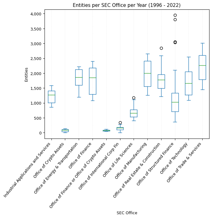
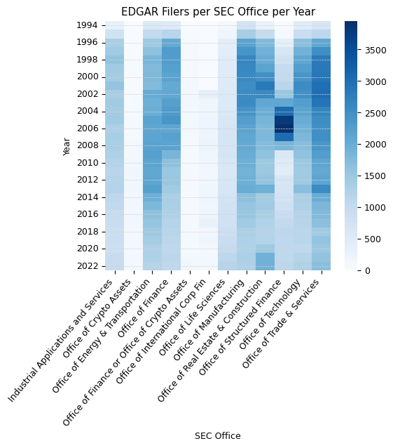
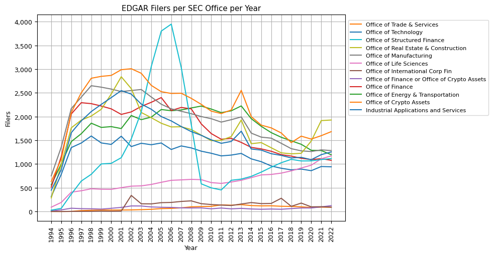
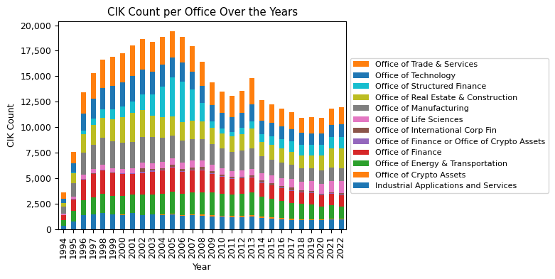
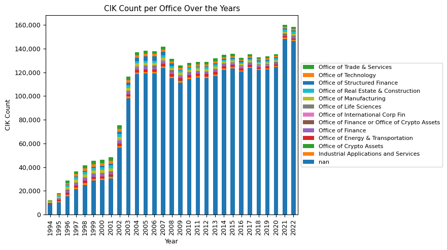
In analyzing the EDGAR filers per SEC Office over the years, several interesting trends emerge. First and foremost, it's evident that the majority of filers is not associated with a SIC code and therefore not associated with an SEC Office. Historically, in 1994, 70% of all filers were not associated with a SIC code. By 2022, this number has surged to 92%. Such a large proportion of filers not being associated with an SEC Office raises the question of who is responsible for overseeing these filers and their filings at the SEC.

To provide context, persons reporting security acquisitions/disposals (Form 3, 4, 5) are not associated with a SIC code. However, they are still mandated to file with the SEC and are subsequently included as an entity in the EDGAR filer data. Given that Form 3/4/5 filings account for around 25% of all filings filed annually, this might shed light on the high number of filers not associated with a SIC code. Yet, it only accounts for a fraction of the 92% of filers without a SIC code.

Delving deeper into specific SEC Offices, the Office of Life Sciences has shown consistent growth, while offices like the Office of Energy & Transportation, Office of Finance, and Office of Technology have seen a mostly consistent decline. The Office of Structured Finance, in particular, peaked around 2005 before witnessing a sharp decline and then stabilizing after 2010. On the other hand, the Office of Crypto Assets, starting from a modest base, has displayed growth, underscoring the rising interest or activity in crypto assets over the years. The dynamics of these trends reflect shifts in sectors or focus areas over the years and can be crucial for understanding the evolving landscape of financial filings.

sic_stats = entities.groupby(['year', 'sic'], dropna=False).cik.count().reset_index(name='cik_count')
sic_stats_pivot = sic_stats.pivot(index='year', columns='sic', values='cik_count')
sic_stats_pivot.fillna(0, inplace=True)
sic_stats_pivot = sic_stats_pivot.loc[:, sic_stats_pivot.mean() >= 50]
sic_stats_pivot = sic_stats_pivot.astype(int)

sic_stats_pivot[-5:]

sic	NaN	0000	1000 Metal Mining	1040 Gold and Silver Ores	1311 Crude Petroleum & Natural Gas	1381 Drilling Oil & Gas Wells	1382 Oil & Gas Field Exploration Services	1400 Mining & Quarrying of Nonmetallic Minerals (No Fuels)	1531 Operative Builders	2834 Pharmaceutical Preparations	...	7372 Services-Prepackaged Software	7373 Services-Computer Integrated Systems Design	7374 Services-Computer Processing & Data Preparation	7389 Services-Business Services, NEC	7990 Services-Miscellaneous Amusement & Recreation	8200 Services-Educational Services	8731 Services-Commercial Physical & Biological Research	8742 Services-Management Consulting Services	8880 American Depositary Receipts	9995 Non-Operating Establishments
year
2018	121854	83	143	116	318	40	40	47	55	658	...	307	59	125	194	33	49	39	79	68	9
2019	122429	69	134	133	285	40	34	49	46	693	...	333	53	131	207	38	57	37	75	136	12
2020	124425	58	111	113	243	31	25	43	55	715	...	323	46	140	194	47	61	34	73	56	16
2021	148279	56	107	120	243	34	34	39	50	797	...	375	48	167	212	44	72	36	69	56	18
2022	146489	69	102	119	197	26	25	37	28	835	...	405	53	176	219	48	76	32	76	46	8

5 rows × 56 columns

top_20_sics_2022 = sic_stats[sic_stats['year'] == 2022].sort_values(by='cik_count', ascending=False)[:10]
top_20_sics_2022

	year	sic	cik_count
12624	2022	NaN	146489
12536	2022	6189 Asset-Backed Securities	1115
12557	2022	6770 Blank Checks	1098
12287	2022	2834 Pharmaceutical Preparations	835
12578	2022	7372 Services-Prepackaged Software	405
12561	2022	6798 Real Estate Investment Trusts	390
12525	2022	6022 State Commercial Banks	253
12523	2022	5990 Retail-Retail Stores, NEC	248
12289	2022	2836 Biological Products, (No Diagnostic Subst...	240
12584	2022	7389 Services-Business Services, NEC	219

sic_stats_wo_nan = sic_stats_pivot.drop(columns=[np.nan, '0000'])

sns.heatmap(sic_stats_wo_nan, cmap='Blues')
plt.gcf().set_size_inches(13, 5)
plt.title("CIK Count per SIC Over the Years"), plt.ylabel("Year"), plt.xlabel("SIC")
plt.gca().yaxis.grid(color='lightgrey', linestyle='dashed', linewidth=0.5)
ax = plt.gca()
ax.set_xticklabels(ax.get_xticklabels(), ha='left')
plt.xticks(np.arange(len(sic_stats_wo_nan.columns)), sic_stats_wo_nan, rotation=90)
plt.show()

sns.heatmap(sic_stats_wo_nan.loc[2009:2022], cmap='Blues')
plt.gcf().set_size_inches(13, 4)
plt.title("CIK Count per SIC Over the Years"), plt.ylabel("Year"), plt.xlabel("SIC")
plt.gca().yaxis.grid(color='lightgrey', linestyle='dashed', linewidth=0.5)
ax = plt.gca()
ax.set_xticklabels(ax.get_xticklabels(), ha='left')
plt.xticks(np.arange(len(sic_stats_wo_nan.columns)), sic_stats_wo_nan, rotation=90)
plt.show()